Next: Loop Corrections
Up: Effective Actions in 4D
Previous: Effective Actions in 4D
Let us consider first the couplings generated at string tree-level
and also tree-level in the sigma-model expansion [34,35].
Besides the 4D Poincaré symmetry, supersymmetry and
gauge symmetries which determine the Cremmer et al Lagrangian,
we also can use the `axionic' symmetry:
 This is a symmetry which for the 4D fields would
imply that
This is a symmetry which for the 4D fields would
imply that  can be shifted by an arbitrary imaginary constant.
There are also two scaling properties of the 4D Lagrangian
can be shifted by an arbitrary imaginary constant.
There are also two scaling properties of the 4D Lagrangian
 ,
,
 for which the Lagrangian
scales as
for which the Lagrangian
scales as
 .
Also, given a scale
.
Also, given a scale  , define
 where
where  gives Newton's constant in 10D. The transformations
 ,
,
 with similar transformations for the other fields, imply that the
Lagrangian should scale as
with similar transformations for the other fields, imply that the
Lagrangian should scale as
 . These scaling properties are not symmetries of the
Lagrangian but of the classical field equations and so
they can be used to restrict the form of the
tree-level effective action only.
. These scaling properties are not symmetries of the
Lagrangian but of the classical field equations and so
they can be used to restrict the form of the
tree-level effective action only.
Using these symmetries we can extract the full dependence of the
effective action on the dilaton field  , which is the most
generic field in all compactifications. We conclude that at tree-level
in both expansions [35]:
, which is the most
generic field in all compactifications. We conclude that at tree-level
in both expansions [35]:
With  still undetermined.
This is however a very crude approximation. What we really want
is to know these functions at tree-level in the string expansion but
exact in the sigma model expansion. This should be
achievable because many of the 4D models are exact
2D CFTs as we saw in the previous chapter.
We can still extract very useful information from
equation (18).
As we said above, the axionic symmetries imply
that to all orders in sigma-model
expansion the superpotential does not depend on
still undetermined.
This is however a very crude approximation. What we really want
is to know these functions at tree-level in the string expansion but
exact in the sigma model expansion. This should be
achievable because many of the 4D models are exact
2D CFTs as we saw in the previous chapter.
We can still extract very useful information from
equation (18).
As we said above, the axionic symmetries imply
that to all orders in sigma-model
expansion the superpotential does not depend on
 and it is just a cubic function of the matter fields
 . This is important for several reasons:
First, we know the field
. This is important for several reasons:
First, we know the field  comes from the internal components of
the metric and controls the loop expansion of the worldsheet
action. If
comes from the internal components of
the metric and controls the loop expansion of the worldsheet
action. If  does not depend on it means that it cannot get
any corrections in sigma model perturbation theory! [23]. Therefore
the only dependence of the (exact) tree-level
superpotential is due to nonperturbative effects in the worldsheet, in particular
all nonrenormalizable couplings in the superpotential are exponentially suppressed (
does not depend on it means that it cannot get
any corrections in sigma model perturbation theory! [23]. Therefore
the only dependence of the (exact) tree-level
superpotential is due to nonperturbative effects in the worldsheet, in particular
all nonrenormalizable couplings in the superpotential are exponentially suppressed ( )[36].
A way to see that there are nonperturbative worldsheet corrections to the
string tree-level superpotential is to realize that
the axionic symmetry shifting by an imaginary constant,
is broken by nonperturbative worldsheet
effects to
)[36].
A way to see that there are nonperturbative worldsheet corrections to the
string tree-level superpotential is to realize that
the axionic symmetry shifting by an imaginary constant,
is broken by nonperturbative worldsheet
effects to
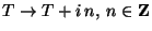 .
This is nothing but
one of the
.
This is nothing but
one of the
 transformation for toroidal orbifold
compactifications (
transformation for toroidal orbifold
compactifications (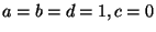 in eq. (10)). Therefore the only conditions these symmetries impose on
is that it should transform as a modular form of a given weight
(
in eq. (10)). Therefore the only conditions these symmetries impose on
is that it should transform as a modular form of a given weight
(
 for the simplest toroidal orbifolds with
the overall size of the compactification space)[37].
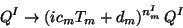
In fact, explicit calculations for specific orbifold models show that
for the simplest toroidal orbifolds with
the overall size of the compactification space)[37].
In fact, explicit calculations for specific orbifold models show that
 |
(19) |
with  a particular modular form of
  or any other duality group
and the ellipsis
represent higher powers of
or any other duality group
and the ellipsis
represent higher powers of  , exponentially suppressed.
The identification of with modular forms was a highly nontrivial
check of the explicit orbifold calculations which were preformed in refs.
[38] without any relation (nor knowledge) of the
underlying duality symmetry . This kind of symmetry
puts also strong constraints to the higher order,
nonrenormalizable, corrections to , since each matter field transforms in a particular way under that symmetry
(
, exponentially suppressed.
The identification of with modular forms was a highly nontrivial
check of the explicit orbifold calculations which were preformed in refs.
[38] without any relation (nor knowledge) of the
underlying duality symmetry . This kind of symmetry
puts also strong constraints to the higher order,
nonrenormalizable, corrections to , since each matter field transforms in a particular way under that symmetry
(
 with
with  the modular weight of ).
There are also other discrete symmetries, as those defined by the point
group
the modular weight of ).
There are also other discrete symmetries, as those defined by the point
group  and space group
  of an orbifold which have
to be respected by the superpotential . These `selection rules' are
very important to find vanishing couplings and uncover flat directions
which can be used to break the original gauge symmetries and
construct quasi-realistic models.
of an orbifold which have
to be respected by the superpotential . These `selection rules' are
very important to find vanishing couplings and uncover flat directions
which can be used to break the original gauge symmetries and
construct quasi-realistic models.
Second, and more important, the superpotential above does not depend
on which is the string loop-counting parameter, and therefore
 does not get renormalized in string perturbation theory!
[39]. This
means that we only need to compute at the tree level and it
will not be changed by radiative corrections. This is the string version of the standard non-renormalization theorems of supersymmetric theories.
Also for
does not get renormalized in string perturbation theory!
[39]. This
means that we only need to compute at the tree level and it
will not be changed by radiative corrections. This is the string version of the standard non-renormalization theorems of supersymmetric theories.
Also for  the superpotential vanishes, independent of the values of
(
the superpotential vanishes, independent of the values of
(
 )! There are not self
couplings among the `moduli' fields and therefore they represent
flat directions in field space
(see for instance [40] ). Notice that due to the non-renormalization theorems, this result is exact in string perturbation theory!.
The only possibilty we have to lift this vacuum degeneracy is by
nonperturbative string effects.
)! There are not self
couplings among the `moduli' fields and therefore they represent
flat directions in field space
(see for instance [40] ). Notice that due to the non-renormalization theorems, this result is exact in string perturbation theory!.
The only possibilty we have to lift this vacuum degeneracy is by
nonperturbative string effects.
The quantity we have less information on, even at tree-level, is the
Kahler potential  . It has been computed only for several
simple cases. For instance in the simplest possible Calabi Yau
compactification (
. It has been computed only for several
simple cases. For instance in the simplest possible Calabi Yau
compactification (
 ) a consistent
truncation from the 10D action gives [34]:
) a consistent
truncation from the 10D action gives [34]:
 |
(20) |
Curiously enough, the second term appeared in the so-called
`no-scale models' studied before string theory [41].
This form holds also for the untwisted fields of orbifold compactifications,
but the dependence on the twisted fields is not known.
It also gives the appropriate result in the large
radius limit of Calabi-Yau compactifications although
it gets non-perturbative worldsheet corrections relevant at
small radii.
In order to find the exact tree-level Kähler potential,
the best that has been done so far is to write the
Kähler potential as an expansion in the matter fields [83]:
and compute the moduli dependent quantities  .
This has been done explicitly for some
.
This has been done explicitly for some  orbifold
compactifications.
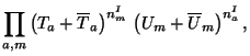
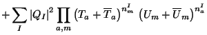
For instance for factorized orbifolds,
that is orbifolds of
a 6D torus which is the product of three 2D tori
orbifold
compactifications.
For instance for factorized orbifolds,
that is orbifolds of
a 6D torus which is the product of three 2D tori  ,
the dependence on the corresponding moduli
fields is given by
,
the dependence on the corresponding moduli
fields is given by
and
 . Giving rise to the Kahler potential:
Where the fractional numbers  are the
`modular weights' of the fields
are the
`modular weights' of the fields  with respect to the
duality symmetries related to the moduli
with respect to the
duality symmetries related to the moduli  or
or  .
For instance, under duality, the fields transform as:
.
For instance, under duality, the fields transform as:
 |
(24) |
Furthermore, for (Calabi-Yau) models, there is
a very interesting observation
[43]. Since these compactifications are also
compactifications of type II strings, and in that case
the corresponding 4D theory has  supersymmetry, the moduli
dependent part of the Kähler potential, has to have the
same dependence as for the models which are much more restrictive.
This underlying structure has been very fruitful to extract
information on models and comes with the name of
`special geometry'.
This restricts the function
supersymmetry, the moduli
dependent part of the Kähler potential, has to have the
same dependence as for the models which are much more restrictive.
This underlying structure has been very fruitful to extract
information on models and comes with the name of
`special geometry'.
This restricts the function  which gives the metric in the moduli
space. First, the moduli space
of the
which gives the metric in the moduli
space. First, the moduli space
of the  forms and the
  forms
forms  factorizes and so:
 |
(25) |
For which the eq. (22) is a particular case.
Second,
in supergravity, the full Lagrangian is
completely determined by a single holomorphic function, the prepotential. The Kähler potential for the fields is a function of the
prepotential  , given by [44]:
 |
(26) |
Where on the right hand side, the subindices mean
differentiation. A similar expression holds for  in terms of a second
prepotential
in terms of a second
prepotential  .
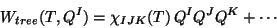
Furthermore, the moduli dependence of the cubic terms
in the superpotential
.
Furthermore, the moduli dependence of the cubic terms
in the superpotential
 |
(27) |
is also given by the functions and since the
Yukawa couplings are given by

Since  and
and  are holomorphic, they may get similar constraints as
the superpotential above.
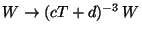
In particular, since
counts sigma model loops, then
are holomorphic, they may get similar constraints as
the superpotential above.
In particular, since
counts sigma model loops, then  is not renormalized
and so
the
is not renormalized
and so
the  dependent part
of the Kähler potential
dependent part
of the Kähler potential
 is given exactly by the
tree-level result!. Similarly, the Yukawa couplings
is given exactly by the
tree-level result!. Similarly, the Yukawa couplings
 are exact at tree-level.
Here is where the mirror symmetry explained in the previous
section plays an important role. Since by mirror symmetry
we understand that the compactification on the original manifold
are exact at tree-level.
Here is where the mirror symmetry explained in the previous
section plays an important role. Since by mirror symmetry
we understand that the compactification on the original manifold
 and its mirror
  represent the
same CFT, and so the same string model, in the version
with the manifold , the roles of and
are interchanged, therefore, computing the dependent part
of the Kähler potential in
(which is exact at tree level) gives the
dependent part of the Kähler potential in !
This fact has been used to compute explicitly the
moduli dependent part of the Kähler potential in some
examples. This overcomes the Calabi-Yau
problem of not knowing the exact CFT behind the
compactification, at least for these couplings.
represent the
same CFT, and so the same string model, in the version
with the manifold , the roles of and
are interchanged, therefore, computing the dependent part
of the Kähler potential in
(which is exact at tree level) gives the
dependent part of the Kähler potential in !
This fact has been used to compute explicitly the
moduli dependent part of the Kähler potential in some
examples. This overcomes the Calabi-Yau
problem of not knowing the exact CFT behind the
compactification, at least for these couplings.
Next: Loop Corrections
Up: Effective Actions in 4D
Previous: Effective Actions in 4D
root
2001-01-22