


Next: Spectrum of the Bosonic
Up: STRINGS, BRANES AND DUALITY1
Previous: Introduction
In this section we overview some basic aspects of bosonic and fermionic
strings. We focus mainly in the description of the spectrum of the theory
in the light-cone gauge, the effective action, the description of spectra of
the five consistent superstring theories and the perturbative Calabi-Yau
compactifications (for details, precisions and further
developments see for instance [3,4,5,6,7,8]).
First of all consider, as usual, the action of a relativistic point
particle. It is given by
 , where
  are
are  functions
representing the coordinates of the
functions
representing the coordinates of the  -dimensional Minkowski spacetime
(the target space),
-dimensional Minkowski spacetime
(the target space),
 and
and
 can be identified with the mass of
the point
particle. This action is
proportional
to the length of the world-line of the relativistic particle.
In analogy with the relativistic point particle, the action describing the dynamics of a
string (one-dimensional object) moving in a -dimensional Minkowski spacetime (the
target space) is proportional to the area
can be identified with the mass of
the point
particle. This action is
proportional
to the length of the world-line of the relativistic particle.
In analogy with the relativistic point particle, the action describing the dynamics of a
string (one-dimensional object) moving in a -dimensional Minkowski spacetime (the
target space) is proportional to the area  of the worldsheet
  . We know from the
theory of surfaces that such an area is given by
. We know from the
theory of surfaces that such an area is given by
 , where
 is
the induced metric (with signature
is
the induced metric (with signature  ) on the worldsheet . The background metric will be
denoted by
) on the worldsheet . The background metric will be
denoted by  and
and
 with
with  are the local
coordinates on the worldsheet. and
are the local
coordinates on the worldsheet. and  are related by
 with
with
 .
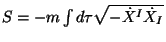
Thus
the classical action of a relativistic string is given by the Nambu-Goto action
.
Thus
the classical action of a relativistic string is given by the Nambu-Goto action
![\begin{displaymath}
S_{NG}[X^{I}]=- T \int_{\Sigma} d\tau d\sigma
\sqrt{-det({\partial}_a X^{I} {\partial}_b X^{J} \eta_{IJ})},
\end{displaymath}](img21.gif) |
(1) |
where
 is the string tension,
  are embedding
functions of the worldsheet into
the target space
are embedding
functions of the worldsheet into
the target space  . Now introduce a metric
  describing the intrinsic worldsheet geometry,
we get a classically equivalent action to the Nambu-Goto action. This is the Polyakov action
originally proposed by Brink, di Vecchia, Howe and Zumino
describing the intrinsic worldsheet geometry,
we get a classically equivalent action to the Nambu-Goto action. This is the Polyakov action
originally proposed by Brink, di Vecchia, Howe and Zumino
![\begin{displaymath}
S_P[X^I,h_{ab}] = - {1\over 4 \pi {\alpha}'} \int_{\Sigma} ...
...igma
\sqrt{-h}h^{ab}\partial_a X^I \partial_b X^J \eta_{IJ},
\end{displaymath}](img26.gif) |
(2) |
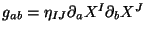
where the 's are scalar fields on the worldsheet. Such a fields can be interpreted
as the coordinates of spacetime (target space), = det and
and
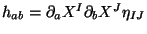 .
Polyakov action has the following symmetries:
.
Polyakov action has the following symmetries:  Poincaré invariance,
 Worldsheet diffeomorphism invariance, and
  Weyl invariance
(rescaling invariance). The energy-momentum tensor of the two-dimensional
theory is given by
Weyl invariance
(rescaling invariance). The energy-momentum tensor of the two-dimensional
theory is given by
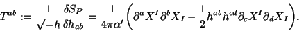 |
(3) |
Invariance under worldsheet diffeomorphisms implies that it should be conserved
i.e.
 , while the Weyl invariance gives the traceless condition,
 . The equation of motion associated with Polyakov action is given by
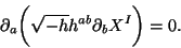 |
(4) |
Whose solutions should satisfy the boundary conditions for the open string:
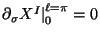 (Neumann) and for the closed
string:
(Neumann) and for the closed
string:
 (Dirichlet). Here
  is
the
characteristic
length of the open string. The variation of
is
the
characteristic
length of the open string. The variation of  with respect to
  leads
to the constraint equations:
leads
to the constraint equations:  .
From now on we will work in the conformal gauge. In this gauge:
.
From now on we will work in the conformal gauge. In this gauge:
 the equations of motion (4) reduce to the Laplace equation in the flat worldsheet
whose solutions can be written as linear superposition of plane waves.
truecm
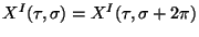
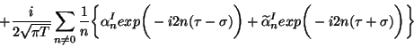
The Closed String
For the closed string the boundary condition
, leads to the general solution of Eq. (4) in the conformal gauge
the equations of motion (4) reduce to the Laplace equation in the flat worldsheet
whose solutions can be written as linear superposition of plane waves.
truecm
The Closed String
For the closed string the boundary condition
, leads to the general solution of Eq. (4) in the conformal gauge
 |
(5) |
where  and
and  are the position and momentum of the
center-of-mass of the string and
are the position and momentum of the
center-of-mass of the string and  and
and
 satisfy the conditions
 (left-movers) and
 (right-movers).
truecm
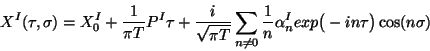
The Open String
For the open string the corresponding boundary condition is
(this is the only boundary condition which is Lorentz invariant) and the solution
is given by
(right-movers).
truecm
The Open String
For the open string the corresponding boundary condition is
(this is the only boundary condition which is Lorentz invariant) and the solution
is given by
 |
(6) |
with the matching condition
 truecm
Quantization
The quantization of the closed bosonic string can be carried over, as usual, by using the Dirac
prescription to the center-of-mass and oscillator variables in the form
truecm
Quantization
The quantization of the closed bosonic string can be carried over, as usual, by using the Dirac
prescription to the center-of-mass and oscillator variables in the form
![\begin{displaymath}[{\alpha}^{I}_m,\widetilde{\alpha}^{J}_n]=0.
\end{displaymath}](img52.gif) |
(7) |
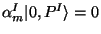
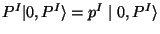
One can identify
 with the annihilation
operators
and the corresponding operators
with the annihilation
operators
and the corresponding operators
 with
the
creation ones. In order to specify the physical states we first denote the center of mass
state given by
with
the
creation ones. In order to specify the physical states we first denote the center of mass
state given by  . The vacuum state is defined by
 with
with  and
and
 and similar for the right movings (here
 ). For the zero modes these states have negative
norm (ghosts). However one can choice a suitable gauge where ghosts decouple from the Hilbert
space when
). For the zero modes these states have negative
norm (ghosts). However one can choice a suitable gauge where ghosts decouple from the Hilbert
space when  .
truecm
Light-cone Quantization
Now we turn out to work in the so called light-cone gauge. In this
gauge it is possible to solve explicitly the Virasoro constraints: . This is done
by removing the light-cone coordinates
.
truecm
Light-cone Quantization
Now we turn out to work in the so called light-cone gauge. In this
gauge it is possible to solve explicitly the Virasoro constraints: . This is done
by removing the light-cone coordinates
 leaving only the transverse coordinates
  representing the physical
degrees of freedom (with
representing the physical
degrees of freedom (with
 ). In this gauge the Virasoro constraints
are explicitly
solved. Thus the independent variables are
). In this gauge the Virasoro constraints
are explicitly
solved. Thus the independent variables are
 . Operators
  and
and
 can be written in terms of
  and
and
 respectively as
follows:
respectively as
follows:
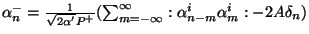 and
and
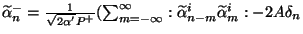 ). For the
open string we get
). For the
open string we get
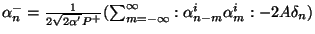 . Here
  stands for the normal ordering and
  is its associated constant.
In this gauge the Hamiltonian is given by
is its associated constant.
In this gauge the Hamiltonian is given by
 |
(8) |
where  is the operator number,
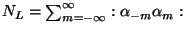 , and
, and
 The
mass-shell condition is given by
The
mass-shell condition is given by
 (open string) and
 (closed string). For the open string,
Lorentz invariance implies that the first excited state is massless and therefore
(closed string). For the open string,
Lorentz invariance implies that the first excited state is massless and therefore  . In the
light-cone
gauge takes the form
. In the
light-cone
gauge takes the form
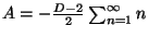 .
From the fact
.
From the fact
 where
where  is the Riemann's zeta function (which converges for
  and has a unique analytic continuation at
 , where it takes the value
  ) then
 and therefore .
truecm
and therefore .
truecm
Subsections
Next: Spectrum of the Bosonic
Up: STRINGS, BRANES AND DUALITY1
Previous: Introduction
root
2001-01-15